What to do with "null" results - Part II: Nonsignificant but with sufficient data

 

What to do with "null" results

Part II: Nonsignificant but with sufficient data

PREAMBLE

• I assume you have some familiarity with frequentist stats and NHST
• I will default to general conventions to avoid unnecessary verbiage (e.g., "p > .05" instead of saying "a p-value higher than your per-selected alpha criterion for long-run Type I error control")
• When possible, I will explain a concept briefly instead of just pointing to a 300+ page statistics book, but with the implied risk my explanation will be limited.
• this is a guide (i explain something) not a tutorial (i show you how to do it); I can do a tutorial if people want (let me know in the comments)
• I will only use open license software to explain concepts, but no R code unless I have to; I know people might just want to implement solutions with things like JASP and G*Power directly.
  

PREMISE

I continue the series of what to do with nonsignificant (aka. "null") results. In this post, I tackle the common situation where although you were successful in collecting all the data you anticipated you needed (i.e., you met your planned N), you still find a p-value over the significance threshold. So, what do you do next?

As before, one thing you shouldn't do is report "there is no effect of X, p>.05". And as before, this is both wrong and incomplete. In this post, I will explain why and what you should report instead.

MAIN

In Part I, I illustrated how precarious the situation in which you have both a nonsignificant results and an underpowered study can be for making causal inferences. However, I advocate that even in such scenarios there is useful information to report, and if you follow a few simple steps and use the proper techniques (e.g., estimation statistics) you can add to the scientific literature. 

However, what if everything went right and you were able to collect sufficient data, what does a non-significant result mean and what inferences can you draw?

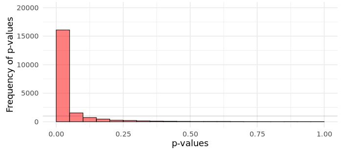
A little recap on NHST and frequentist statistics (see longer explanation in Part I) to make sure we are all on the same page. A while back there was huge scandal on Twitter and the blogosphere regarding proper interpretations of p-values (see here). This boils down to remembering that under the Neyman-Pearson hypothesis testing framework (the one were we specify alpha levels, statistical power, effect sizes, and sample sizes) we cannot interpret the p-value as a measure of evidence for the Null. This might be shocking to many, as a common - but wrong - interpretation of p-values is that they reflect the probability of the null hypothesis being true. They do not. For a simplistic and incomplete explanation of why this is, you just need to understand that if there really is no effect (0), i.e., the null hypothesis is true, then the probability of ANY p-value is equally likely! Namely, under the null, the distribution of p-values is uniform:

Fig. 1 Distribution of p-values from 20,000 simulated experiments when there is no effect (i.e., null is true). Simulated using this Shiny app here

 

 

What this means is that if there is "no effect", obtaining a p = .001 is just as likely as p = .999! That might seem confusing at first given that we seem to care so much about p < .05 in research (which is a problem onto itself, but I digress). Here is why we use some predetermined alpha: if all possible values of P are equally probable, we know how often we are likely to observe a value within a specific range, namely between .00-.05. It's 5% of the time. If we choose alpha < .025, then it's 2.5% of the time, if we chose alpha < .72, then it's 72% of the time, and so on. (And to understand how arbitrary this is, we could also pick values between .20-.25 as the target range - even if it make no senses - and we would still only observe p-values in that range 5% of the time if the null is true) This is why you often see statistics textbooks write this sentence "the probability of observing the data or more extreme data given a hypothesis is true" [emphasis added]. You are essentially saying "interpreting a p-value smaller than .05 as if there is an effect could mean I'm wrong, but I shouldn't be wrong, in the long run, more than 5% of the time".

(TBH, I think a lot of the confusion surrounding the p-value comes from journals requiring we report the exact value obtained, e.g.,  p = .002, instead of the older version of simply stating p < .05; the latter is correct for the N-P approach, but we realised that people were p-hacking their data, or outright misinterpreting the real value, so the decision was made to report it in full. There are other concerns I don't cover here, like the Jeffreys-Lindley paradox, that justify reporting the actual value, but in terms of decision-making, focusing on binary (or ternary; Neyman & Pearson, 1933) test outcome is valid.)

This is why Neyman and Pearson argued that we need to also consider the Alternative Hypothesis (Ha) to make sense of the data, and why we need to carefully consider what the difference (effect or relationship) might be beforehand. P-values only allow you to say how often your results would reflect a false positive by setting an acceptable percentage of long-run error (e.g., 5%). But, it says nothing about your long-run error for making a false negative (i.e., missing a finding). For that you need to determine the effect size you anticipate reflects reality (e.g., smallest effect size of interest, SESOI, or the minimum detectable effect, MDE), and ensure you would have sufficient data to detect such an effect at a set probability (i.e., statistical power). For simplicity, say you anticipate the true difference between your two conditions is a Cohen's d = .40. You now need to say "how often do I want to be able to detect this effect, in the long run, if it exists?" If you say 80% of the time, that is your power and you plan your sample size accordingly. This is what this state of the world looks like:

Fig. 2 Distribution of p-values from 20,000 experiments that have a sample size large enough to detect a true effect size (d = .40) 80% of the time, in the long run.

The above figure shows the possible distribution of p-values if there is an effect. The tallest red bar represent the proportion of p-values that are under our alpha of 5%. It is 80% of all p-values simulated. That is what statistical power is: the long-run proportion of p-values that would fall under your alpha threshold if the effect of the size you predict exists.

So, if you didn't consider your effect size a priori, and your didn't set a power threshold, and you didn't collect the sample size that would allow you to reliably detect your anticipated difference then the p-value tells you very little.

Scenario 2: Everyone did your study, but your p-value is high 😓 (nonsignificant, but sufficiently powered)

Assuming you are all caught up on the above, and you wanted to run an experiment to detect a difference of d = .40 between two conditions. You run an a priori power analysis (independent samples comparison, two-tailed, at α = 0.05, and power = 80%, for a d = .40) which computes an N = 200 (n = 100 per condition). If all you plan for in terms of sample size and power relates to this Ha it is only half the battle. You need to also plan for accepting no effect. But, as we just covered, that cannot be done based on a single statistical test. Alongside your anticipated effect you also need to consider a range of values that are practically equivalent to "no effect". This is what Equivalence Tests are for, and it is arguably what you need to actually plan your sample size around.

For a primer on Two One-Sided Test (TOST) of equivalence, see Lakens (2017). The way the testing procedure is used can seem a bit contrived at first, so I will provide a rough guide to how it works. Simply, overlooking the testing itself, you can see it as a method of determining if the effect you obtain in a study and its associated uncertainty falls within a region of values we can take as zero (too small to care) or outside it (big enough to care).

Fig. 3 Illustration of the 4 different scenarios relating to TOST equivalence tests; taken from Lakens (2017)

In the current blog I only cover 2 of the outcomes displayed in the above figure, to avoid confusion or making this too long (A and D). I do recommend the paper to gain a proper understanding of what is going on, but in essence what the NHST + TOST approach to inference aims to achieve is determining if the p > .05 obtained in a study can be attributed to an effect being too small to matter (i.e., indistinguishable from a "zero" region - dotted lines above; outcome A) or due to a high level of uncertainty (e.g., outcome D).

For designing your study, you have two options: (1) your study uses a SESOI, so all values below it are considered "no effect", or (2) your target effect (d = .40) is separate from what you define as a negligible difference (e.g., -.20 < d < .20). In (1), your sample size should reflect a TOST that has equivalence bounds around -.39 < d < .39 (i.e., just smaller than your SESOI). In (2), your sample size focuses on being able to reliably accept "no effect", and your equivalence bounds are, -.20 < d < .20.

If we compute power (at 80%) for the above scenarios we see the following:

1. To detect a d = .40 you need N = 200, but your power for the TOST is only 73%; the sample needed for the TOST is N = 228  (n = 114). So, you should collect N = 228 (n = 114).
2. To detect a d = .40 you need N = 200, as above, but to power for the TOST of ±.20 you need an N = 860 (n = 430)!
   

(The above calculations were done using the TOSTER package; but for an excellent overview and some easy-to-use suggestion on sample sizes, see Brysbaert, 2019.)

This illustrates a serious problem in research that is often ignored: we need much larger samples that we often see in published work to make sense of the data (at least for frequentists; Bayesians can quantify anything). That said, if your SESOI is all that you would consider, then it is clear planning for 80% power to detect it would still permit a decent TOST procedure.

What to do and what to report:

 For (1), I expect that your Method section reads like this for Sample:

"An a priori power analysis for an independent samples comparison, two-tailed, at α = 0.05 and power = 80%, for a SESOI of d = .40, determined that 200 participants needed to be recruited; Control (n = 100) and Treatment (n = 100). All effects below this threshold (d < .40) are taken as negligible. To ensure sufficient statistical power for a TOST procedure, a sample of N = 228 was required."

 For (2), I expect that your Method section reads like this for Sample:

"An a priori power analysis for an independent samples comparison, two-tailed, at α = 0.05 and power = 80%, considering a typical effect size in this area / replication attempt / etc. of a d = .40, determined that 200 participants needed to be recruited; Control (n = 100) and Treatment (n = 100). Given the exploratory nature of the investigation, to also ensure that the study has sufficient data to exclude all theoretically/clinically relevant effect sizes, the final sample size was determined considering a TOST procedure for excluding non-negligible effects with equivalence bounds of d =±.20. The estimated sample size needed is N = 860 (n = 430 per condition)."

The above is to make sure you have some guidance on what a power analysis for such research would look like. While these procedures have been around for decades, they are rarely employed in psychology. I hope the example text reduces some of the barriers for researchers to employ these approaches in their own work.

Outcome A Now, in your Results section, I will imagine two scenarios. First, I will start with outcome A in Fig.3 - you obtain a p > .05 and the effect is "equivalent to zero".

Let's say you collected N = 228 participants, everything went well, and then you run a Student's t-test to assess if there is a statistically significant difference in your sample. You run the test and, oops!, t(226) = -0.54, p = 0.590, Hedges' g = -0.07, 95% CI [-0.33, 0.19]. So, your test statistic was not significant. But, at this point you can't conclude much. You don't yet know if this result reflects no effect, high uncertainty, or a false negative (all 3 possibilities are valid without further testing).

To be able to claim that there is "no effect" of the manipulation on the outcome you need to conduct a TOST. You can run a TOST either using the TOSTER package, JASP, or Jamovi. I won't go into the details of what the procedure does, as the wording always leads to more confusion (just read the cited paper above). Briefly, it tests if your data are within the boundary region of equivalence you specified (which you should have done a priori in a pre-registration). One t-test looks at the upper bound, and one at the lower bound. If your effect estimate is within this region, both tests with have p < .05 (yes, it works in reverse to the normal hypothesis test; I told you it's confusing).

For this data the output is like this: Upper TOST, ΔU, t(226) = -3.45,  p < 0.001, significant result. Lower TOST, ΔL, t(226) = 2.37, p = 0.009, significant result. As both tests are statistically significant, it implies the data (i.e., estimated effect) lies fully within the region of equivalence (see Fig.4), leading to the conclusion of statistically equivalent and not different. Namely, you can claim "no effect".

Fig. 4 Outcome A: Equivalence plot for the standardised effect size estimate (g) of the difference between Control and Treatment. The dotted lines represent the region of equivalence (i.e., values inside are taken as "zero effect")

For write-up you would say:

 "Participants in the Control condition (M = 100, SD = 70, n = 114) show a pattern of lower health scores than participants in the Treatment condition (M = 105, SD = 70, n = 114), Mdiff = -5.00, SE = 9.27, Hedges' g = -0.07, 95% CI [-0.33, 0.19]. A Student's independent samples t-test comparing the scores in the two conditions found a non-significant result, t(226) = -0.54, p = 0.590. Thus, the null hypothesis cannot be rejected. A two one-sided test (TOST) of equivalence was conducted to discern if the result reflects no effect or insufficient data. The TOST, using equivalence bounds of ±27 points (d = ±0.39), yielded a significant result for the lower bound, ΔL, t(226) = 2.37, p = 0.009, and a significant result for the upper bound, ΔU, t(226) = -3.45, p < 0.001. This is interpreted as statistically equivalent and not different (i.e., no effect of the manipulation)."

For the discussion, you can now infer that there is no effect:

"The Hypothesis of a difference in Health outcome between the two conditions was not supported, with the difference between the Control and Treatment condition falling entirely within the region of equivalence. This suggests no effect of the manipulation."

Outcome D The second possible outcome is D in Fig.3 - you obtain a p > .05 and the data is to uncertain to make a firm conclusion. 

In this scenario, you were also able to collect N = 228, and then you ran the t-test and found a non-significant result, t(226) = -1.94, p = 0.053, Hedges' g = -0.26, 95% CI [-0.52, 0.01]. Now, you run a TOST to see if this non-significant result implies no effect or high uncertainty.

For this data the output is like this: Upper TOST, ΔU, t(226) = -4.85,  p < 0.001, significant result. Lower TOST, ΔL, t(226) = 0.97, p = 0.166, non-significant result. This time, one of the t-tests is non-significant, meaning we cannot exclude meaningful effect sizes from our data. This result is interpreted as not equivalent and not different  (i.e., insufficient data to draw a conclusion). Looking at Fig 5. it is clear that the left tail of the effect estimate crosses the equivalence bound reaching -.52 (at 95% CI; or -.47, at 90% CI), which is big enough in magnitude as a potential effect to consider meaningful. Thus, this is an example of when a p > .05 tells us very little about our hypothesis.

Fig. 5 Outcome D: Equivalence plot for the standardised effect size estimate (g) of the difference between Control and Treatment. The dotted lines represent the region of equivalence (i.e., values inside are taken as "zero effect")

For write-up you would say:

 "Participants in the Control condition (M = 100, SD = 70, n = 114) show a pattern of lower health scores than participants in the Treatment condition (M = 118, SD = 70, n = 114), Mdiff = -18.00, SE = 9.27, Hedges' g = -0.07, 95% CI [-0.52, 0.01]. A Student's independent samples t-test comparing the scores in the two conditions found a non-significant result, t(226) = -1.94, p = 0.053. Thus, the null hypothesis cannot be rejected. A two one-sided test (TOST) of equivalence was conducted to discern if the result reflects no effect or insufficient data. The TOST, using equivalence bounds of ±27 points (d = ±0.39), yielded a significant result for the upper bound, ΔU, t(226) = -4.85, p < 0.001, but a non-significant result for the lower bound, ΔL, t(226) = 0.97, p = 0.166. This is interpreted as not equivalent and not different (i.e., insufficient data to draw a conclusion)."

For the discussion, you cannot infer no effect, and must conclude that the current data is too uncertain:

"The current data is too uncertain for a firm conclusion to be drawn. The estimated difference between the two conditions, while non-significant, has large uncertainty, with the data being compatible with negligible improvements in health outcomes (.01), no effect (0), but also with large and theoretically relevant decreases in health outcomes (-.52). Thus, more research using a larger sample or different operationalisation is needed."

And that is it. A bit long in the tooth, but this topic is rather nuanced and has many moving parts. Hopefully, the above provides some useful insight and guidance on what to do and report in your research. For an example paper using the above approaches, see my preprint:

Zloteanu, M. (2022, December 20). Uncertain Veracity Judgements: Does the Framing of the Question Influence Deception Detection?. https://doi.org/10.31234/osf.io/wrsgn

Footnotes:

Astute readers of the equivalence outcome figure will identify that C refers to an interesting scenario that we don't see mentioned often: a difference can be statistically significant (does not cross 0) but still too small to matter (all compatible values are within the region of equivalence). This is a common occurrence with studies that have huge sample sizes, as any non-zero deviation will reach significance.

Above I mention that a p > .05 from a hypothesis test can reflect no effect, high uncertainty, or a false negative, and that TOST can solve this issue. That is only partly correct, as your results may still be due to a false negative (it will happen 20% of the time). As I mentioned in Part I, you shouldn't put too much stock into a single experiment. For now, based on the results you would just act as if there is no effect, until you have reason to change your view. If it was important research, maybe increase power in the future to, say, 95%.

The purpose of this post was to cover equivalence tests, however, the testing part is not strictly necessary. As shown in Part I, you can make inferences about an effect using the 95% CIs. If the CI of the effect falls entirely within the SESOI equivalence bounds (i.e., -δ, δ), you may conclude a negligible / no effect. This is why plotting your data is always useful.

References:

Brysbaert, M. (2019). How many participants do we have to include in properly powered experiments? A tutorial of power analysis with reference tables. Journal of Cognition, 2(1), 16. DOI: http://doi.org/10.5334/joc.72

Lakens, D. (2017). Equivalence Tests: A Practical Primer for t Tests, Correlations, and Meta-Analyses. Social Psychological and Personality Science, 8(4), 355–362. https://doi.org/10.1177/1948550617697177 

Neyman, J., & Pearson, E. S. (1933). The testing of statistical hypotheses in relation to probabilities a priori. Mathematical Proceedings of the Cambridge Philosophical Society, 29(04), 492–510. https://doi.org/10.1017/S030500410001152X